sunshine> matlab

                              < M A T L A B >
                  Copyright 1984-1999 The MathWorks, Inc.
                        Version 5.3.1.29215a (R11.1)
                                Oct  6 1999

  To get started, type one of these: helpwin, helpdesk, or demo.
  For product information, type tour or visit www.mathworks.com.

>>
Check out the demos sometime. To get the online help (in your Netscape browser) type "doc" at the prompt. There is a very good on-line tutorial, which you should work through. Just click "Getting Started" in the help.
Let's start by entering a 4x4 matrix and calling it A:
>> A=[16 3 2 15; 15 10 11 8; 9 6 7 12; 4 15 14 1]

A =

    16     3     2    15
    15    10    11     8
     9     6     7    12
     4    15    14     1
Let's ask Matlab for its transpose:
>> A'

ans =

    16    15     9     4
     3    10     6    15
     2    11     7    14
    15     8    12     1

>>
We will now enter a 4-dimensional row vector, and try to form the products bA and Ab:
>> b=[ 1.4 5.23 1.22 -1.1]

b =
    1.4000    5.2300    1.2200   -1.1000

>> b*A

ans =

  107.4300   47.3200   53.4700   76.3800

>> A*b
??? Error using ==> *
Inner matrix dimensions must agree.

>>
Of course, we can multiply a 4-dimensional row vector on the right by a 4x4 matrix, but not on the left. If we enter a 4-dimensional column vector, we can left multiply, but not right multiply:
>> b=[ 1.4; 5.23; 1.22; -1.1]

b =

    1.4000
    5.2300
    1.2200
   -1.1000

>> A*b

ans =

   24.0300
   77.9200
   39.3200
  100.0300

>> b*A
??? Error using ==> *
Inner matrix dimensions must agree.

>>
Suppose we want to solve the equation Av=b. Formally the solution is v=A-1b, so we need to divide b by A on the left. We'll do this now, and then check by computing Av and Av-b.
>> v=A\b

v =

    0.5070
   -1.4192
    1.3214
   -0.3398

>> A*v

ans =

    1.4000
    5.2300
    1.2200
   -1.1000

>> A*v-b

ans =

   1.0e-14 *

    0.1332
    0.1776
    0.0666
    0.3553
Note that the last answer is not exactly zero. There is rounding error. The rounding error is very small; Matlab works to about 16 figure accuracy, but usually only prints 4 digits after the decimal point.
If we make b a row vector again, we can try to solve b=wA. The solution is w=bA-1, so we need to divide b on the right by A:
>> b=[ 1.4 5.23 1.22 -1.1]

b =
    1.4000    5.2300    1.2200   -1.1000

>> w=b/A

w =

    1.1283   -0.7273   -1.1046    1.0497

>> w*A

ans =

    1.4000    5.2300    1.2200   -1.1000

>> w*A-b

ans =

   1.0e-14 *

    0.0444         0   -0.1110         0
Here's a shortcut to produce a row vector with the entries 0,1,2,...,10:
>> t=0:10

t =

     0     1     2     3     4     5     6     7     8     9    10

>>
If we want a row vector with entries 0,0.1,0.2,...9.9,10.0 we can get it with
>> t=0:0.1:10;

>>
Note I have supressed output by finishing the line with a ;
Most functions in Matlab work componentwise on matrices. So we can do
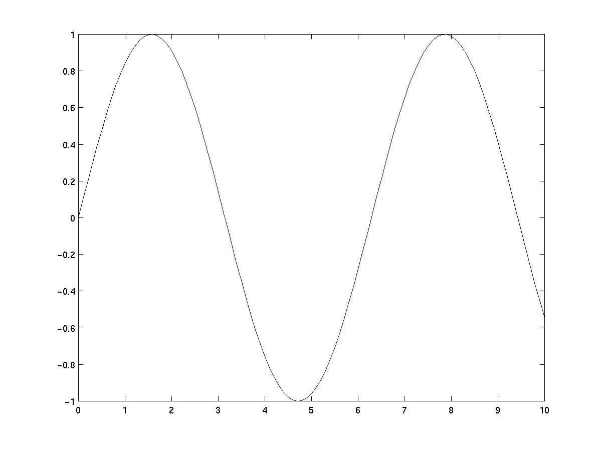
>> y=sin(t);

>>
and the supressed output will be 101-dimensional vector with the values of sin(t) in for t = 0,0.1,0.2,..10.0. We can now get a graph of sin(t) by plotting y against t:
>> plot(t,y)

>>
The output appears in another window, and looks like this:
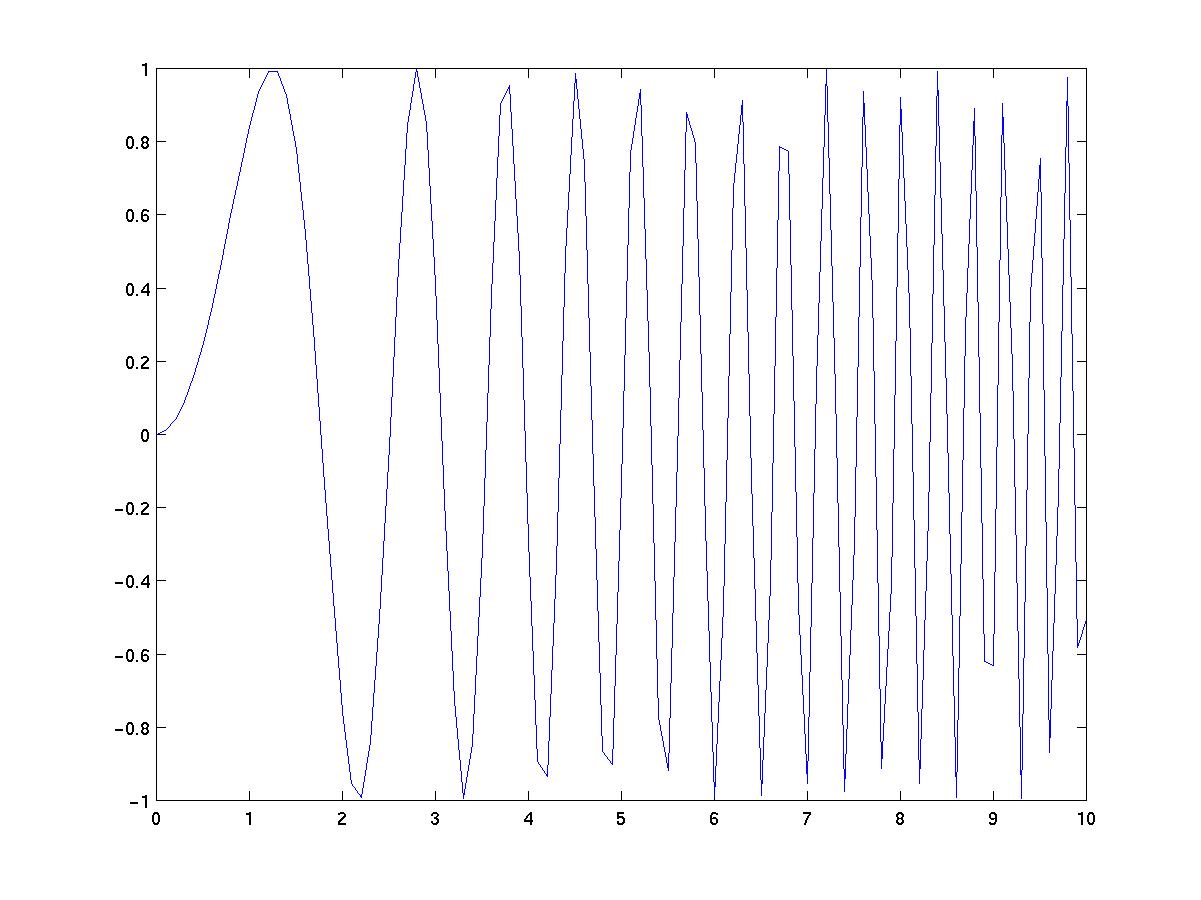
What if I want the graph of sin(t2)? First try:
>> z=sin(t*t);
??? Error using ==> *
Inner matrix dimensions must agree.

>>
t is a row vector and so this tried to multiply two vectors, which fails. We need "component-wise multiplication" using .*:
>> z=sin(t.*t);

>> plot(t,z)

>>
The result is:
In the Getting Started section of the Online Help you can find more details on basic graphics, which is important stuff.
Now, it is a pain to type input to Matlab after the prompt sign, particularly if the same or similar input is used several times. But in fact you can use files for input. These files are called "M files" and must have names that end with ".m". They must sit in your working directory. In fact there are two types of M files, those used for input, and those used to define functions.
A=[ 16  3  2  15; 15  10  11  8;  9  6  7  12;  4 15  14  1]
b=[ 1.4; 5.23; 1.22;  -1.1]
v=A\b
The if in my Matlab session I type "input1" I get the following response:
>> input1

A =

    16     3     2    15
    15    10    11     8
     9     6     7    12
     4    15    14     1


b =

    1.4000
    5.2300
    1.2200
   -1.1000


v =

    0.5070
   -1.4192
    1.3214
   -0.3398

>>
Matlab reads and executes all commands in the file input1.m.
function a=func1(x)
a = (1-exp(x)*sin(x)+x^3) / (x*tan(x)+1/2)
This then defines a new Matlab function called func1. If I try to call it by typing "func1(2)" at the prompt, the following happens
>> func1(2)

a =

   -0.5894

ans =

   -0.5894

>>
The function works, but prints an intermediate result which we should have supressed. Another problem arises if we try to apply it to a vector:
>> func1([1 2])
??? Error using ==> *
Inner matrix dimensions must agree.

Error in ==> func1.m
On line 2  ==> a= (1-exp(x)*sin(x)+x^3) / (x*tan(x)+1/2)
We should have defined the operations in the function to be component operations. So let's change the file to
function a=func1(x)
a= (1-exp(x).*sin(x)+x.^3) ./ (x.*tan(x)+1/2);
Suppose now I want to find the roots of func1, i.e. the points x such that func1(x)=0. We do
>> x=-2:0.02:2;
>> plot(x,func1(x))
to get
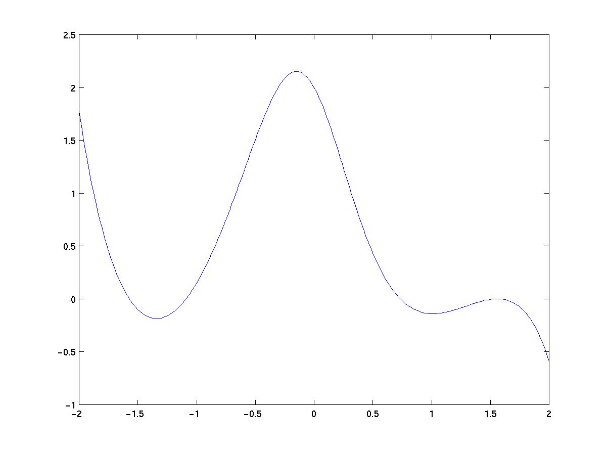
One root is (I guess) between -1.6 and -1.5. Let's track it down by interval bisection:
>> func1(-1.6)

ans =

    0.0533

>> func1(-1.5)

ans =

   -0.0994

>> func1(-1.55)
ans =

   -0.0335

>> func1(-1.575)

ans =

    0.0072

>> func1(-1.5625)

ans =

   -0.0138

>> func1(-1.56875)

ans =

   -0.0035

>> func1(-1.571875)

ans =

    0.0018
Let's automate this procedure. The function below in the file bisec1.m inputs a 2-vector a1 which is the initial interval that contains the root, and an integer n which is the number of times we want to bisect this interval:
function a2=bisec1(a1,n)

% interval bisection to find roots of func1(x)=0
% input a1 is a two-vector [a,b] in which a root lies

f=func1(a1);

for i=1:n
   mid=(a1(1)+a1(2))/2;
   midf=func1(mid);
   if (midf*f(1)>0)
        a1(1)=mid;
        f(1)=midf;
     else
        a1(2)=mid;
        f(2)=midf;
   end
end

a2=a1;
Some new things in this function: calling a vector's components, the for loop syntax (note the "end"), the if syntax (note the "end"), comments.
Problems with this function: does it work if you land exactly on zero? What other problems can you spot?
Here is a run of this program starting from the by hand results and doing 30 more bisections.
>> bisec1([-1.571875,-1.56875],30)

ans =

   -1.5708   -1.5708
The accuracy of the presentation is insufficient here. We already had the root accurate to within about 0.003, and each 10 bisections improves accuracy by a factor of 1000. We need to do:
>> format long
>> bisec1([-1.571875,-1.56875],30)

ans =

  -1.57079632679524  -1.57079632679233

>>
Exercise: find the other roots visible on the graph, each to 12 figure accuracy.
For more information on matlab you should look at the extensive online help (type "doc") or one of the numerous manuals that are available on the internet, see here for some links.