Scilab/Matlab program for polynomial interpolation and some examples

Polynomial interpolation is not a very common thing these days (splines are preferred), so I had to write my own little scilab program to do it. The function "inter" defined below takes two input (row) vectors, the first is interpreted as the x-coordinates of the points to be interpolated, the second as the y-coordinates. The output is a plot of the data and the interpolating polynomial.

For Shira's Matlab version, click here.


function inter(X,Y)

// find size of data, minimum and maximum x

n=size(X,2);
least=X(1);
most=X(1);
for i=2:n 
   if (X(i)<least)
      least=X(i)
   end
   if (X(i)>most)
      most=X(i)
   end
end 

// make table of divided differences

table=zeros(n,n);
table(:,1)=Y';
for i=2:n
for j=i:n
table(j,i)=(table(j,i-1)-table(j-1,i-1))/(X(j)-X(j-i+1));
end
end

// make graph of polynomial using Horner's method and plot

x=[0:100]*(most-least)/100+least;
y=table(n,n);
for i=1:(n-1)
   y=y.*(x-X(n-i))+table(n-i,n-i);
end
xbasc(0)
plot2d(X,Y,style=-4)
plot2d(x,y,style=4)

endfunction

Here are some examples of runs:

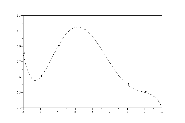
X=[10 9 8 4 2 3]               // the x-coordinates need not be ordered
Y=[0.1 0.3 0.4 0.9 0.8 0.5]
inter(X,Y)

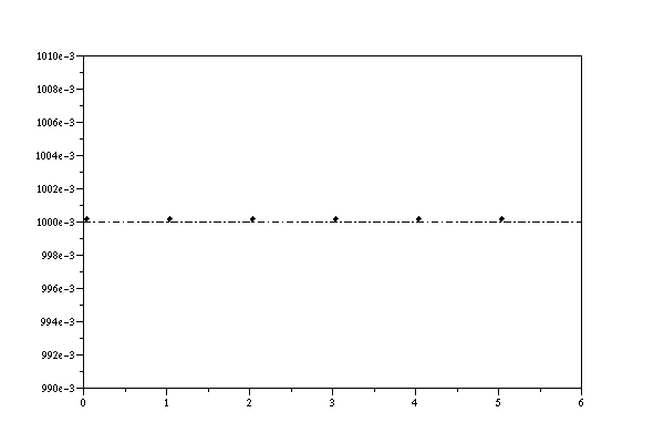
X=[0 1 2 3 4 5 6]
Y=[1 1 1 1 1 1 1]          // straight line output expected
inter(X,Y)

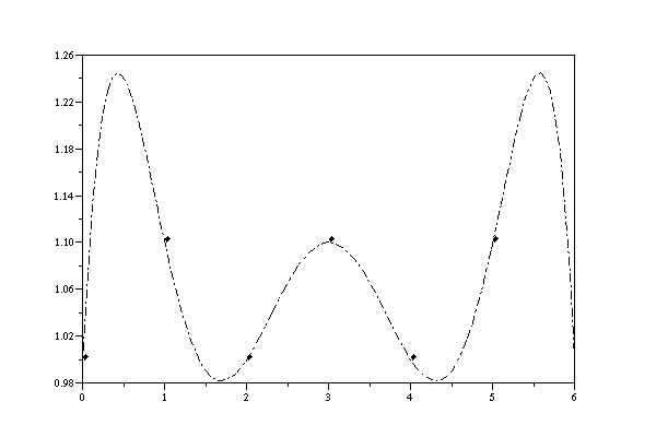
X=[0 1 2 3 4 5 6]
Y=[1 1.1 1 1.1 1 1.1 1]
inter(X,Y)

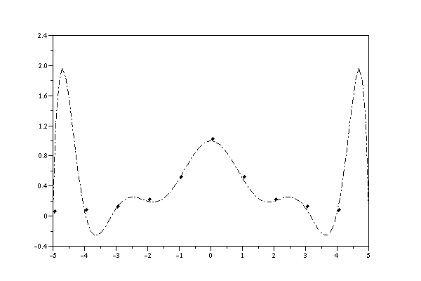
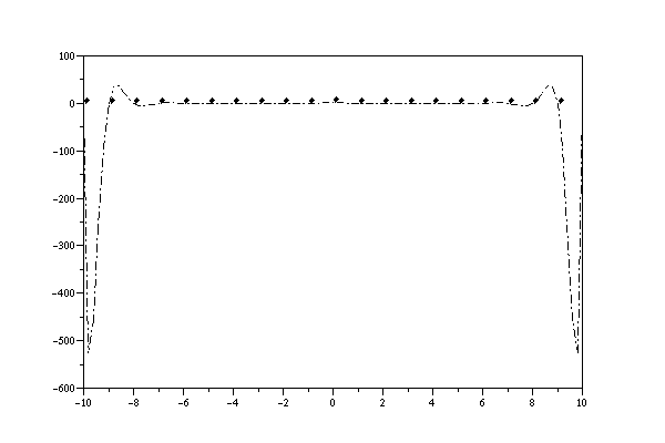
Polynomial interpolation can give highly oscillatory results if the x-coordinates are equally spaced apart. The classic example of this is known as "Runge's example". We try to do polynomial interpolation of equally spaced points on the curve y=1/(1+x^2). Below are results using 11 and 21 points:

X=[-5:5]
Y=(X.*X+1).^(-1)   
inter(X,Y)

X=[-10:10]
Y=(X.*X+1).^(-1)   
inter(X,Y)

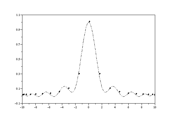
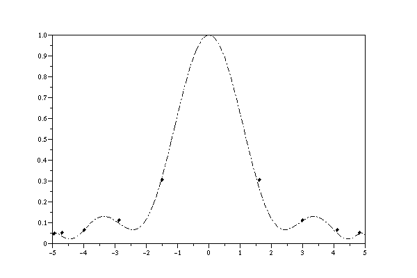
To cure this we need to squash the points up a bit towards the end of the ends of the interpolation interval. Here is a better way to do it, using 11 and 21 respectively:

X=5*sin(%pi*[-5:5]/10)
Y=(X.*X+1).^(-1)   
inter(X,Y)

X=10*sin(%pi*[-10:10]/20)
Y=(X.*X+1).^(-1)   
inter(X,Y)