sunshine> matlab

                              < M A T L A B >
                  Copyright 1984-1999 The MathWorks, Inc.
                        Version 5.3.1.29215a (R11.1)
                                Oct  6 1999

  To get started, type one of these: helpwin, helpdesk, or demo.
  For product information, type tour or visit www.mathworks.com.

>>
Check out the demos sometime. To get the online help (in your Netscape browser) type "doc" at the prompt. There is a very good on-line tutorial, which you should work through. Just click "Getting Started" in the help.
Matlab can be used to do what a calculator does. For example:
>> 1/29 + 1/31

ans =

    0.0667

>> asin(1/2)

ans =

    0.5236

>> exp(i*pi)

ans =

  -1.0000 + 0.0000i
Note that by default matlab works to about 16 figure accuracy, but it only prints 5 digit answers.
However, Matlab is far more powerful than simple calculator! The main advantage of Matlab is that it makes matrix manipulations easy. Let's start by entering a 4x4 matrix and calling it A:
>> A=[16 3 2 15; 15 10 11 8; 9 6 7 12; 4 15 14 1]

A =

    16     3     2    15
    15    10    11     8
     9     6     7    12
     4    15    14     1
Let's ask Matlab for its transpose:
>> A'

ans =

    16    15     9     4
     3    10     6    15
     2    11     7    14
    15     8    12     1

>>
We will now enter a 4-dimensional row vector, and try to form the products bA and Ab:
>> b=[ 1.4 5.23 1.22 -1.1]

b =
    1.4000    5.2300    1.2200   -1.1000

>> b*A

ans =

  107.4300   47.3200   53.4700   76.3800

>> A*b
??? Error using ==> *
Inner matrix dimensions must agree.

>>
Of course, we can multiply a 4-dimensional row vector on the right by a 4x4 matrix, but not on the left. If we enter a 4-dimensional column vector, we can left multiply, but not right multiply:
>> b=[ 1.4; 5.23; 1.22; -1.1]

b =

    1.4000
    5.2300
    1.2200
   -1.1000

>> A*b

ans =

   24.0300
   77.9200
   39.3200
  100.0300

>> b*A
??? Error using ==> *
Inner matrix dimensions must agree.

>>
Suppose we want to solve the equation Av=b. Formally the solution is v=A-1b, so we need to divide b by A on the left. We'll do this now, and then check by computing Av and Av-b.
>> v=A\b

v =

    0.5070
   -1.4192
    1.3214
   -0.3398

>> A*v

ans =

    1.4000
    5.2300
    1.2200
   -1.1000

>> A*v-b

ans =

   1.0e-14 *

    0.1332
    0.1776
    0.0666
    0.3553
Note that the last answer is not exactly zero. There is a small rounding error.
If we make b a row vector again, we can try to solve b=wA. The solution is w=bA-1, so we need to divide b on the right by A:
>> b=[ 1.4 5.23 1.22 -1.1]

b =
    1.4000    5.2300    1.2200   -1.1000

>> w=b/A

w =

    1.1283   -0.7273   -1.1046    1.0497

>> w*A

ans =

    1.4000    5.2300    1.2200   -1.1000

>> w*A-b

ans =

   1.0e-14 *

    0.0444         0   -0.1110         0
Here's a shortcut to produce a row vector with the entries 0,1,2,...,10:
>> t=0:10

t =

     0     1     2     3     4     5     6     7     8     9    10

>>
If we want a row vector with entries 0,0.1,0.2,...9.9,10.0 we can get it with
>> t=0:0.1:10;

>>
Note I have supressed output by finishing the line with a ;
Most functions in Matlab work componentwise on matrices. So we can do
>> y=sin(t);

>>
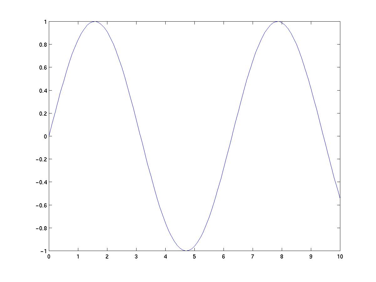
and the supressed output will be 101-dimensional vector with the values of sin(t) in for t = 0,0.1,0.2,..10.0. We can now get a graph of sin(t) by plotting y against t:
>> plot(t,y)

>>
The output appears in another window, and looks like this:
What if I want the graph of sin(t2)? First try:
>> z=sin(t*t);
??? Error using ==> *
Inner matrix dimensions must agree.

>>
t is a row vector and so this tried to multiply two vectors, which fails. We need "component-wise multiplication" using .*:
>> z=sin(t.*t);

>> plot(t,z)

>>
The result is:

In the Getting Started section of the Online Help you can find more details on basic graphics, which is important stuff.
Now, it is a pain to type input to Matlab after the prompt sign, particularly if the same or similar input is used several times. But in fact you can use files for input. These files are called "M files" and must have names that end with ".m". They must sit in your working directory. In fact there are two types of M files, those used for input, and those used to define functions.
A=[ 16  3  2  15; 15  10  11  8;  9  6  7  12;  4 15  14  1]
b=[ 1.4; 5.23; 1.22;  -1.1]
v=A\b
The if in my Matlab session I type "input1" I get the following response:
>> input1

A =

    16     3     2    15
    15    10    11     8
     9     6     7    12
     4    15    14     1


b =

    1.4000
    5.2300
    1.2200
   -1.1000


v =

    0.5070
   -1.4192
    1.3214
   -0.3398

>>
Matlab reads and executes all commands in the file input1.m.
function a=func1(x)
a = (1-exp(x)*sin(x)+x^3) / (x*tan(x)+1/2)
This then defines a new Matlab function called func1. If I try to call it by typing "func1(2)" at the prompt, the following happens
>> func1(2)

a =

   -0.5894

ans =

   -0.5894

>>
The function works, but prints an intermediate result which we should have supressed. Another problem arises if we try to apply it to a vector:
>> func1([1 2])
??? Error using ==> *
Inner matrix dimensions must agree.

Error in ==> func1.m
On line 2  ==> a= (1-exp(x)*sin(x)+x^3) / (x*tan(x)+1/2)
We should have defined the operations in the function to be component operations. So let's change the file to
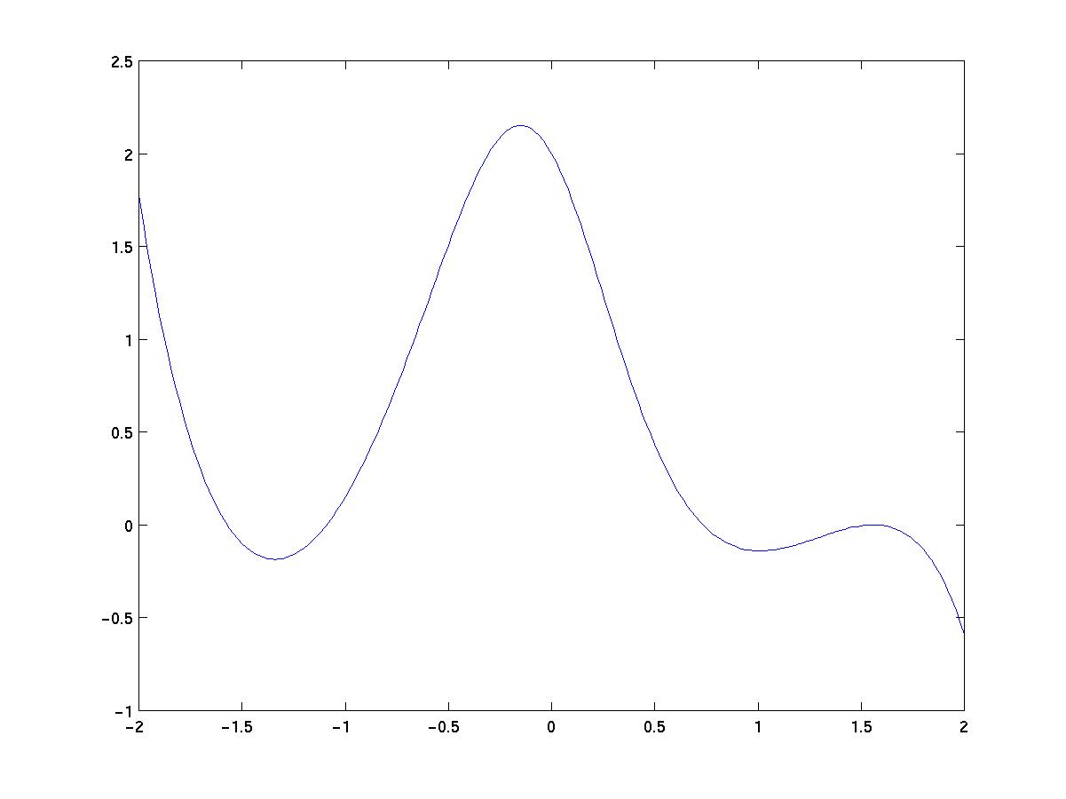
function a=func1(x)
a= (1-exp(x).*sin(x)+x.^3) ./ (x.*tan(x)+1/2);
Now that func1 works on vectors we can plot it. We do
>> x=-2:0.02:2;
>> plot(x,func1(x))
to get
>> [x,y] = meshgrid(-2:.2:2, -2:.2:2);
>>  z = x .* exp(-x.^2 - y.^2);
>>  mesh(x,y,z)
Which give:
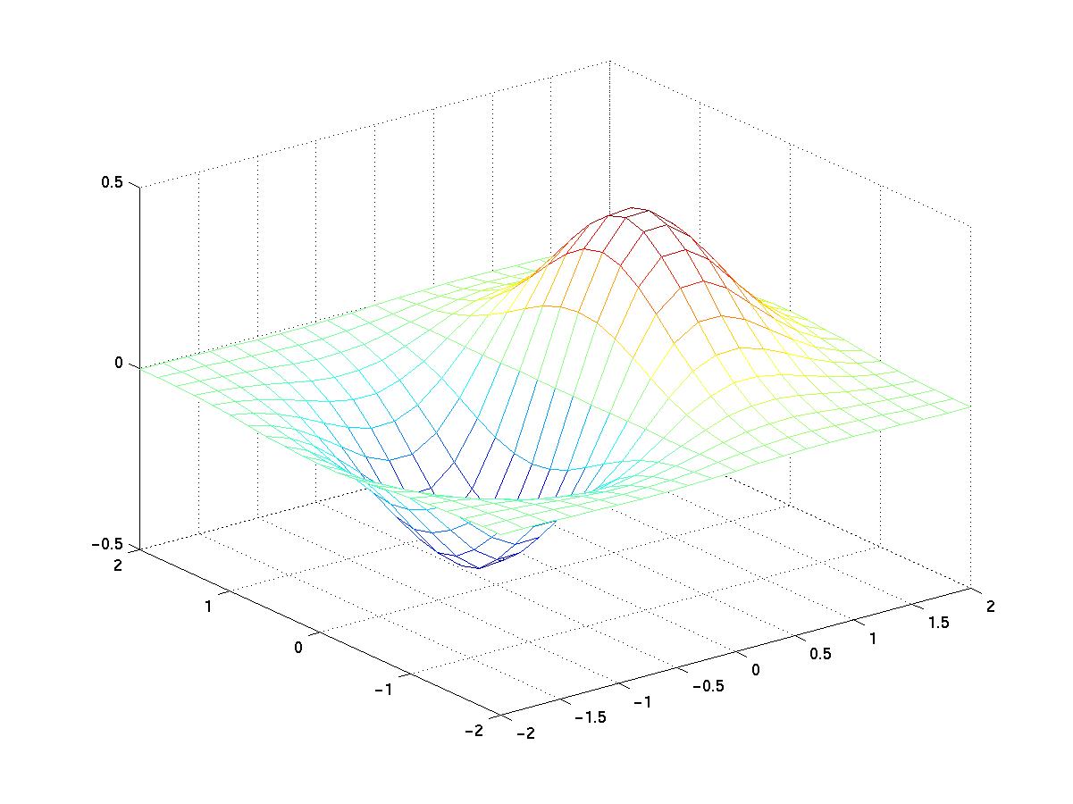
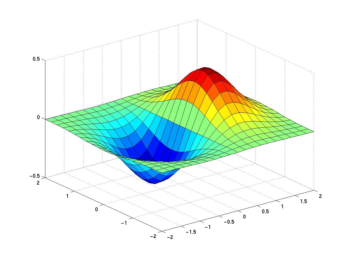
If the
mesh(x,y,z)command is replaced by
surf(x,y,z)the output is
>> x=1/2;
>> for i=1:10
     x=5/2*x*(1-x)
    end
(note you do not get a prompt when you're in the middle of a loop) gives results:
x = 0.6250
x = 0.5859
x = 0.6065
x = 0.5966
x = 0.6017
x = 0.5992
x = 0.6004
x = 0.5998
x = 0.6001
x = 0.5999
Here is a VERY BASIC program for Gaussian elimination. Put it in a file called gelim.m.
function a=gelim(x)
a=x;
m=size(a,1);
n=size(a,2);
for i=1:m-1
  for j=i+1:n
     a(j,:)=a(j,:)-a(j,i)/a(i,i)*a(i,:);
end
end
The code uses the fact that if a is a matrix in matlab then a(i,j) is the i,j-th entry in the matrix. a(i,:) is the i-th row, a(:,j) is the j-th column. size(a,1) tells you the number of rows in a, size(a,2) tells you the number of columns. Check the function works by writing, say,
x=[1 1 1; 2 1 1 ; 0 -3 19]
gelim(x)
Why would it fail if the 2,2-th entry in the above matrix were 2?